Performance
This doc describes the performance-oriented pieces of astropath:
the numpy-accelerated core calculations, the optional numba
acceleration for the fixed-grid posterior, and the profiling
module used to measure them.
numpy-accelerated core
The two most expensive steps in a PATH analysis have been re-implemented in pure numpy:
localization.calc_LWx(the localization term \(L(w-x)\)) for the error-ellipse (eellipse) localization now computes the angular separation and position angle with closed-form numpy formulae instead ofastropySkyCoordoperations. Results are numerically identical (to roundoff) and the routine is several times faster on large grids.bayesian.px_Oi_fixedgrid(the fixed-grid \(p(x|O_i)\)) pre-extracts the candidate and center coordinates into numpy arrays once, rather than readingastropyattributes inside the per-candidate loop.bayesian.px_Oi_local(the local-grid \(p(x|O_i)\), which builds one grid per candidate) has likewise been rewritten in pure numpy for theeellipselocalization: it pre-extracts the coordinates once and evaluates \(L(w-x)\) directly in a flat-sky tangent plane, removing everyastropycall from the per-candidate loop. Other localization types (healpix,wcs) fall back tolocalization.calc_LWxas before. See Local-grid posterior below for details.
These changes are transparent: you do not need to do anything to benefit from them, and the public APIs are unchanged.
Optional numba acceleration
The per-candidate loop of bayesian.px_Oi_fixedgrid can optionally
be evaluated with a numba kernel
(bayesian.px_Oi_numba) that fuses the offset, offset-PDF, product
with \(L(w-x)\), and grid sum into a single pass with no full-grid
temporaries.
To enable it, pass use_numba=True:
from astropath import bayesian

p_xOi = bayesian.px_Oi_fixedgrid(
    box_hwidth, localiz, cand_coords, cand_ang_size,
    theta_prior, step_size=0.1, use_numba=True)
Key points:
Optional.
numbaneed not be installed. If it is absent (or if you simply leaveuse_numba=False, the default), the calculation runs via the standard numpy path. Withuse_numba=Truebutnumbanot installed, the code emits a warning and falls back to numpy — it never errors.Default is off.
use_numbadefaults toFalse, so existing code and results are unchanged unless you opt in.Only ``px_Oi_fixedgrid``. The numba option is available only for the fixed-grid method.
px_Oi_localand the other routines are unaffected. The fused kernel returns only the scalar posterior, so it is bypassed (numpy path used) whenreturn_gridsorreturn_debugis requested.Primarily for sandbox analyses. numba is recommended mainly for interactive/sandbox work and large-grid experiments, where its speed-up is largest. The first call pays a one-time JIT compilation cost; the win grows with the grid size and the number of candidates (roughly 1.5x on small grids up to ~5-6x on a 7200x7200 grid with many candidates).
Note
The numba flag is exposed on bayesian.px_Oi_fixedgrid directly.
The high-level path.PATH.calc_posteriors does not currently
forward use_numba; call bayesian.px_Oi_fixedgrid directly to
use it.
Local-grid posterior
bayesian.px_Oi_local evaluates \(p(x|O_i)\) on a separate grid
per candidate, centered on the galaxy and sized to the offset prior
(box_hwidth = phi*max). It is the method of choice for
localizations that span a large area of sky, where
a single fixed grid would be prohibitively large.
For the eellipse localization the calculation is pure numpy and
flat-sky:
The per-candidate grid is built once in normalized units and merely rescaled per galaxy — the pixel count
ngrid = 2*max/step_sizeis the same for every candidate.\(L(w-x)\) is evaluated directly in the tangent plane (offsets rotated into the ellipse frame), matching the spherical
calc_LWxto ~1e-5 fractionally at arcsec scales.
Here step_size is relative to the galaxy size (default 0.05),
so the grid spacing is phi*step_size.
Note
px_Oi_local is pure numpy and does not require (or use)
numba — for now. The optional numba acceleration described above
applies only to px_Oi_fixedgrid. px_Oi_local is fast on its
own because each per-candidate grid is small.
Small-localization correction
When the localization minor axis \(b\) is smaller than the galaxy
angular size \(\phi\), the galaxy-centered grid under-resolves the
sharp localization and the raw sum is biased low. In that case
px_Oi_local divides the result by a correction factor computed by
bayesian._Lwx_correction: the discrete “total \(L(w-x)\)” on a
small grid that is centered on the localization and aligned to the
galaxy grid (same spacing, shifted by an integer number of cells).
Because the localization is sampled at the same sub-cell phase in the
raw sum and in this factor, the under-resolution bias cancels in the
ratio (accurate to ~1%). This is the local analogue of
px_Oi_fixedgrid’s correction='L_wx'. The correction grid is
bounded (it is skipped when it would exceed ~5000 cells per side, which
only happens when the localization is already well resolved and no
correction is needed), so it never allocates a large array.
Profiling module
The astropath.profiling module measures these calculations across a
range of grid sizes. It mirrors the
calculations/step_size/Profiling.ipynb notebook: a faux FRB, a
circular error ellipse, and a set of candidate galaxies spread over a
range of locations and angular sizes.
Run it from the command line:
python -m astropath.profiling
This sweeps a range of step_size values (hence grid sizes) and
profiles both posterior methods:
calc_LWx, the numpypx_Oi_fixedgrid, and (ifnumbais installed) the numba path with its speed-up factor — written toprofiling_timing.png;px_Oi_local(viarun_profiling_local), whose per-candidate grid size is2*max/step_size— written toprofiling_local_timing.png.
Both timing tables are printed to the screen.
You can also import and call the pieces directly:
from astropath import profiling

df = profiling.run_profiling()            # fixed-grid (+ numba)
profiling.plot_results(df, 'timing.png')

df_local = profiling.run_profiling_local()   # local-grid method
profiling.plot_local_results(df_local, 'local.png')
Benchmark results
Accuracy
px_Oi_local is validated against px_Oi_fixedgrid run on a fine
grid (the astropath/tests/tests_local.py module). Both evaluate the
same integral \(p(x|O_i)=\int L(w-x)\,p(w|O_i)\,dw\); the fine fixed
grid is taken as truth. Across the size regimes the local method
reproduces it to a fraction of a percent (run at step_size=0.02):
Case |
localization |
galaxy |
rel. diff |
|---|---|---|---|
large galaxy / small loc |
a=b=1″ |
10″ |
+7.0e-5 |
large galaxy / large loc |
a=b=10″ |
10″ |
-3.3e-3 |
small galaxy / small loc |
a=b=1″ |
1″ |
-3.3e-3 |
small galaxy / large loc |
a=b=10″ |
1″ |
-3.3e-3 |
small galaxy / ellipse |
a=10″, b=0.2″ |
0.5″ |
-3.3e-3 |
When the localization minor axis is smaller than the galaxy
(\(b<\phi\)) the _Lwx_correction removes the O(step) bias, so the
result stays accurate even at coarse (galaxy-relative) step sizes where
the uncorrected sum would be off by ~1-2 %:
Case |
step |
raw (no corr.) |
corrected |
|---|---|---|---|
gal 10″ / loc a=b=1″ |
0.05 |
-0.85 % |
-1.7e-4 |
gal 10″ / loc a=b=1″ |
0.10 |
-1.85 % |
-1.9e-3 |
ellipse a=10″, b=0.2″ |
0.05 |
-0.84 % |
-7.1e-6 |
ellipse a=10″, b=0.2″ |
0.10 |
-1.66 % |
+3.4e-5 |
Even for a very small (sub-arcsec) localization, where the galaxy grid
badly under-resolves the localization, the correction recovers the fine
fixed-grid value (step_size=0.05):
galaxy |
rel. diff |
|---|---|
0.3″ |
+6.9e-5 |
0.6″ |
+2.5e-5 |
1.0″ |
+4.8e-5 |
Profiling
Timings below were produced by python -m astropath.profiling (50
candidate galaxies; absolute times are machine-dependent, the trends and
ratios are the point).
Fixed-grid posterior (px_Oi_fixedgrid): the numba path overtakes
numpy beyond small grids, reaching ~5-6x on the largest grids; the
one-off JIT cost makes it slower than numpy only on the smallest grid.
step |
grid |
calc_LWx |
numpy |
numba |
numba speed-up |
|---|---|---|---|---|---|
0.50 |
360² |
9 ms |
30 ms |
145 ms |
0.2x |
0.25 |
720² |
42 ms |
173 ms |
91 ms |
1.9x |
0.10 |
1800² |
344 ms |
2.06 s |
670 ms |
3.1x |
0.05 |
3600² |
1.67 s |
16.4 s |
2.96 s |
5.6x |
0.025 |
7200² |
6.49 s |
68.5 s |
12.4 s |
5.5x |
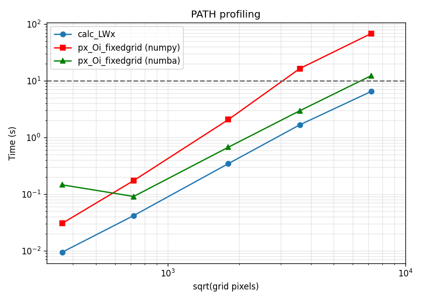
Fixed-grid timing vs grid side length (sqrt of pixels). The dashed line marks 10 s.
Local-grid posterior (px_Oi_local): the cost depends on the
localization. With no correction (circular, \(b\ge\phi\)) or a tiny
localization (a=b=0.1”, small correction grid) the per-candidate cost is
modest; a long thin ellipse (a=12.5”, b=0.2”) drives the correction grid
to ~1000² and dominates the run time – i.e. the correction cost scales
with the localization major axis.
step |
galaxy grid |
ellipse corr grid |
circular |
ellipse |
small loc |
|---|---|---|---|---|---|
0.50 |
24² |
97² |
0.9 |
6.8 |
2.3 |
0.25 |
48² |
197² |
1.8 |
22 |
3.3 |
0.10 |
120² |
497² |
7.9 |
146 |
11 |
0.05 |
240² |
997² |
31 |
1553 |
41 |
0.025 |
480² |
1997² |
155 |
9037 |
185 |
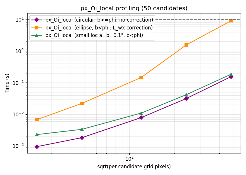
Local-grid timing vs per-candidate galaxy-grid side length, for the three localization scenarios. The dashed line marks 10 s.
API Reference
Profiling utilities for the PATH calculations.
This module times the two core PATH steps that were targeted for the numpy speed-up work (see prompts/speed_up.md):
localization.calc_LWx– the localization term L(w-x)
bayesian.px_Oi_fixedgrid– the fixed-grid p(x|O_i)
It is modeled on the calculations/step_size/Profiling.ipynb
notebook: a faux FRB, a circular error ellipse, and a couple of
candidate galaxies. Rather than timing each sub-step interactively, it
sweeps a range of grid sizes (by varying step_size), builds a table
of timings, prints it, and writes a figure.
Run from the command line:
python -m astropath.profiling
or import and call run_profiling() directly.
- astropath.profiling.default_setup(ncand=50)[source]
Build the faux-FRB profiling scenario.
Mirrors calculations/step_size/Profiling.ipynb (circular 5” error ellipse), but scatters
ncandcandidate galaxies over a range of locations and angular sizes so the per-candidate loop inpx_Oi_fixedgridis exercised realistically.- Parameters:
ncand (int, optional) – Number of candidate galaxies.
- Returns:
- (localiz, cand_coords, cand_ang_size, theta_prior)
localiz (dict): eellipse localization dict. cand_coords (SkyCoord): candidate host coordinates. cand_ang_size (np.ndarray): candidate angular sizes, arcsec. theta_prior (dict): offset-prior parameters.
- Return type:
- astropath.profiling.ellipse_setup(ncand=50)[source]
High-axis-ratio ellipse scenario that exercises _Lwx_correction.
Unlike
default_setup()(circular localization, whereb >= phiso no correction fires), this uses a long thin error ellipse (a=12.5”, b=0.2”, axis ratio ~60) with candidate galaxies LARGER thanb.px_Oi_localtherefore triggers the_Lwx_correctionfor every candidate. The galaxy sizes (1.5”-2.5”) are chosen so the correction grid is ~1000x1000 cells at the default step (0.05) – and stays below the ~5000-cell skip threshold across the whole step sweep.- Parameters:
ncand (int, optional) – Number of candidate galaxies.
- Returns:
- (localiz, cand_coords, cand_ang_size, theta_prior), same
shape as
default_setup().
- Return type:
- astropath.profiling.main()[source]
Run the profiling sweep, print the table, and save the figure.
- Parameters:
None
- Returns:
The timing table (also printed to screen).
- Return type:
- astropath.profiling.plot_local_results(df, outfile)[source]
Plot px_Oi_local timing vs per-candidate grid size (log-log).
- Parameters:
df (pandas.DataFrame) – Output of
run_profiling_local().outfile (str) – Path to write the PNG figure.
- Returns:
The path the figure was written to.
- Return type:
- astropath.profiling.plot_results(df, outfile)[source]
Plot the timing results vs grid size on log-log axes.
- Parameters:
df (pandas.DataFrame) – Output of
run_profiling().outfile (str) – Path to write the PNG figure.
- Returns:
The path the figure was written to.
- Return type:
- astropath.profiling.run_profiling(step_sizes=None, box_hwidth=90.0)[source]
Profile calc_LWx and px_Oi_fixedgrid over a range of grid sizes.
- Parameters:
- Returns:
- One row per step size with columns
step_size,ngrid,n_pixels,calc_LWx_s,px_Oi_fixedgrid_s(numpy) andpx_Oi_numba_s(the numbause_numba=Truepath; NaN if numba is unavailable).
- Return type:
- astropath.profiling.run_profiling_local(step_sizes=None)[source]
Profile px_Oi_local over a range of (relative) step sizes.
px_Oi_localbuilds one grid per candidate, sized to the offset prior (box_hwidth = phi*max) with spacing phi*step_size. The per-candidate pixel count is thereforengrid = 2*max/step_size(independent of phi), so sweepingstep_sizesweeps the per-candidate grid size. The whole multi-candidate call is timed.Three scenarios are timed against this SAME per-candidate galaxy grid (the x-axis of the figure):
circular(default_setup()) –b >= phi, so the_Lwx_correctionnever fires: pure galaxy-grid cost.ellipse(ellipse_setup()) – a long thin localization (a=12.5”, b=0.2”) withb < phi, so the correction fires every candidate on a ~1000x1000 grid (at the default step).small(small_loc_setup()) – a tiny circular localization (a=b=0.1”) with galaxies 0.1”-20”; the correction fires but its grid stays small (tiny major axis). Comparing the three isolates how the correction cost scales with the localization size.
- Parameters:
step_sizes (list, optional) – Relative step sizes to sweep. Defaults to
DEFAULT_STEP_SIZES.- Returns:
- One row per step size with columns
step_size,ngrid(per candidate),n_pixels(per candidate),ncand,px_Oi_local_s(circular),px_Oi_local_ellipse_s(ellipse + correction),px_Oi_local_smallloc_s(small localization), andcorr_ngrid(representative ellipse correction-grid side).
- Return type:
- astropath.profiling.small_loc_setup(ncand=50)[source]
Very small (sub-arcsec) circular localization scenario.
A tiny circular error ellipse (a=b=0.1”) with candidate galaxies spanning 0.1”-20”. For every galaxy larger than
bthe_Lwx_correctionfires, but because the ellipse major axis is tiny its correction grid (~8a/h cells per side) stays small even as the galaxy grid grows – the opposite regime toellipse_setup()(large axis ratio -> large correction grid). This stresses the deeply under-resolved case (grid spacingphi*stepcan be many timesb).- Parameters:
ncand (int, optional) – Number of candidate galaxies.
- Returns:
- (localiz, cand_coords, cand_ang_size, theta_prior), same
shape as
default_setup().
- Return type: