Simulating FRB Populations with astropath
This notebook demonstrates how to use the astropath.simulations.generate_frbs module to generate synthetic FRB populations with realistic properties for different surveys (CHIME, DSA, ASKAP).
The generated FRBs have the following properties:
DM: Extragalactic dispersion measure (pc/cm³)
z: Redshift
M_r: Host galaxy absolute r-band magnitude
m_r: Host galaxy apparent r-band magnitude
[1]:
import numpy as np
import matplotlib.pyplot as plt
import pandas as pd

# Set up plotting style
plt.rcParams['figure.figsize'] = (10, 6)
plt.rcParams['font.size'] = 12
[2]:
from astropath.simulations import generate_frbs, SURVEY_GRIDS
/home/xavier/Projects/FRB/FRB/frb/halos/hmf.py:51: UserWarning: hmf_emulator not imported.  Hope you are not intending to use the hmf.py module..
  warnings.warn("hmf_emulator not imported.  Hope you are not intending to use the hmf.py module..")
Available Surveys
The module supports several FRB surveys, each with its own P(z,DM) grid that captures the selection effects and sensitivity of that instrument.
[3]:
print("Available surveys:")
for survey in SURVEY_GRIDS.keys():
    print(f"  - {survey}")
Available surveys:
  - CHIME
  - DSA
  - ASKAP
  - CRAFT
  - CRAFT_ICS_1300
  - CRAFT_ICS_892
  - CRAFT_ICS_1632
  - Parkes
  - FAST
Basic Usage: Generate FRBs for a Single Survey
The simplest usage generates FRBs by sampling from the survey-specific P(z,DM) grid.
[4]:
# Generate 1000 CHIME FRBs with a fixed seed for reproducibility
df_chime = generate_frbs(1000, 'CHIME', seed=42)

print(f"Generated {len(df_chime)} CHIME FRBs")
df_chime.head(10)
Loading P(DM,z) grid from /home/xavier/Projects/FRB/FRB/frb/data/DM/CHIME_pzdm.npz
Sampling DM values
Sampling redshifts
Sampling host galaxy absolute magnitudes
Using Lz values to sample host galaxy absolute magnitudes
Generated 1000 CHIME FRBs
[4]:
| DMeg | z | M_r | m_r | |
|---|---|---|---|---|
| 0 | 445.0 | 0.25 | -21.681575 | 18.889973 |
| 1 | 1175.0 | 1.38 | -20.278551 | 24.743318 |
| 2 | 710.0 | 0.63 | -18.475358 | 24.456045 |
| 3 | 585.0 | 0.45 | -19.330649 | 22.723243 |
| 4 | 215.0 | 0.11 | -18.918085 | 19.690382 |
| 5 | 215.0 | 0.11 | -19.709010 | 18.899457 |
| 6 | 225.0 | 0.05 | -19.538448 | 17.269064 |
| 7 | 850.0 | 0.94 | -18.647786 | 25.346529 |
| 8 | 1225.0 | 0.45 | -21.433325 | 20.620566 |
| 9 | 930.0 | 0.59 | -20.513442 | 22.245471 |
[5]:
# Summary statistics
df_chime.describe()
[5]:
| DMeg | z | M_r | m_r | |
|---|---|---|---|---|
| count | 1000.000000 | 1000.000000 | 1000.000000 | 1000.000000 |
| mean | 599.490000 | 0.472650 | -20.223130 | 20.900058 |
| std | 476.539431 | 0.435738 | 1.556904 | 3.054551 |
| min | 30.000000 | 0.010000 | -23.336626 | 10.759040 |
| 25% | 280.000000 | 0.160000 | -21.465300 | 18.925289 |
| 50% | 470.000000 | 0.350000 | -20.384238 | 21.014704 |
| 75% | 770.000000 | 0.650000 | -19.179283 | 23.037714 |
| max | 4455.000000 | 3.760000 | -15.189843 | 30.037022 |
Comparing Different Surveys
Different surveys have different selection functions, leading to different redshift and DM distributions. Let’s compare CHIME, DSA, and ASKAP.
[6]:
# Generate FRBs for three major surveys
n_frbs = 5000
seed = 42

df_chime = generate_frbs(n_frbs, 'CHIME', seed=seed)
df_dsa = generate_frbs(n_frbs, 'DSA', seed=seed)
df_askap = generate_frbs(n_frbs, 'ASKAP', seed=seed)

surveys = {
    'CHIME': df_chime,
    'DSA': df_dsa,
    'ASKAP': df_askap
}
Loading P(DM,z) grid from /home/xavier/Projects/FRB/FRB/frb/data/DM/CHIME_pzdm.npz
Sampling DM values
Sampling redshifts
Sampling host galaxy absolute magnitudes
Using Lz values to sample host galaxy absolute magnitudes
Loading P(DM,z) grid from /home/xavier/Projects/FRB/FRB/frb/data/DM/DSA_pzdm.npz
Sampling DM values
Sampling redshifts
Sampling host galaxy absolute magnitudes
Using Lz values to sample host galaxy absolute magnitudes
Loading P(DM,z) grid from /home/xavier/Projects/FRB/FRB/frb/data/DM/CRAFT_class_I_and_II_pzdm.npz
Sampling DM values
Sampling redshifts
Sampling host galaxy absolute magnitudes
Using Lz values to sample host galaxy absolute magnitudes
[7]:
# Compare summary statistics
print("Survey Comparison Summary")
print("=" * 60)
for name, df in surveys.items():
    print(f"\n{name}:")
    print(f"  DM:  median = {df['DMeg'].median():.0f}, range = [{df['DMeg'].min():.0f}, {df['DMeg'].max():.0f}] pc/cm³")
    print(f"  z:   median = {df['z'].median():.3f}, range = [{df['z'].min():.3f}, {df['z'].max():.3f}]")
    print(f"  m_r: median = {df['m_r'].median():.1f}, range = [{df['m_r'].min():.1f}, {df['m_r'].max():.1f}]")
Survey Comparison Summary
============================================================
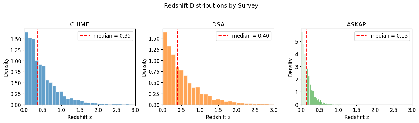
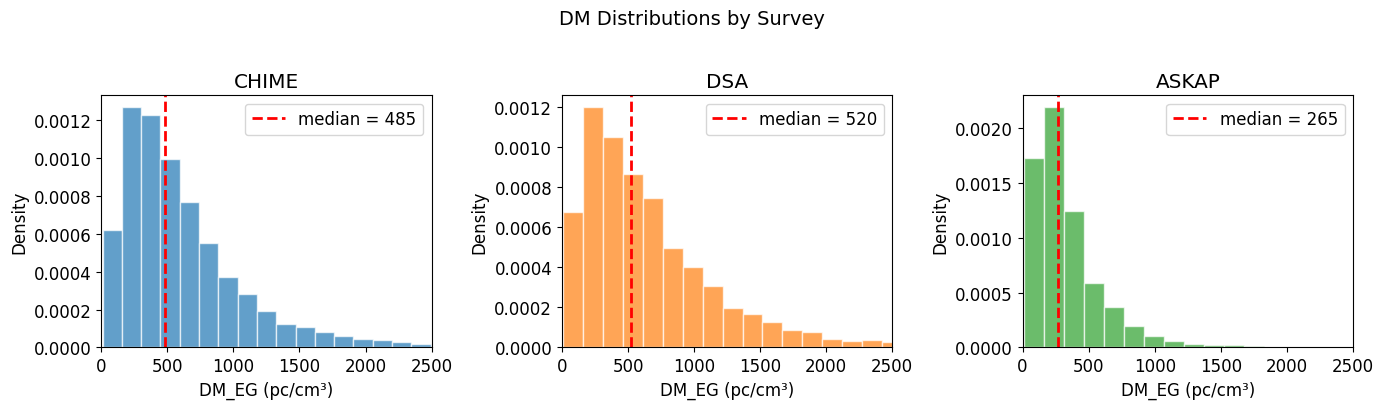
CHIME:
DM: median = 485, range = [10, 5850] pc/cm³
z: median = 0.350, range = [0.010, 3.760]
m_r: median = 21.0, range = [10.2, 29.8]
DSA:
DM: median = 520, range = [10, 6040] pc/cm³
z: median = 0.400, range = [0.010, 4.400]
m_r: median = 21.3, range = [10.2, 30.3]
ASKAP:
DM: median = 265, range = [10, 6055] pc/cm³
z: median = 0.130, range = [0.010, 1.060]
m_r: median = 18.5, range = [10.1, 26.8]
Redshift Distributions
[8]:
fig, axes = plt.subplots(1, 3, figsize=(14, 4))
colors = ['#1f77b4', '#ff7f0e', '#2ca02c']

for ax, (name, df), color in zip(axes, surveys.items(), colors):
    ax.hist(df['z'], bins=40, alpha=0.7, color=color, density=True, edgecolor='white')
    ax.axvline(df['z'].median(), color='red', linestyle='--', linewidth=2, label=f'median = {df["z"].median():.2f}')
    ax.set_xlabel('Redshift z')
    ax.set_ylabel('Density')
    ax.set_title(f'{name}')
    ax.legend()
    ax.set_xlim(0, 3)

plt.suptitle('Redshift Distributions by Survey', fontsize=14, y=1.02)
plt.tight_layout()
plt.show()
DM Distributions
[9]:
fig, axes = plt.subplots(1, 3, figsize=(14, 4))

for ax, (name, df), color in zip(axes, surveys.items(), colors):
    ax.hist(df['DMeg'], bins=40, alpha=0.7, color=color, density=True, edgecolor='white')
    ax.axvline(df['DMeg'].median(), color='red', linestyle='--', linewidth=2, label=f'median = {df["DMeg"].median():.0f}')
    ax.set_xlabel('DM_EG (pc/cm³)')
    ax.set_ylabel('Density')
    ax.set_title(f'{name}')
    ax.legend()
    ax.set_xlim(0, 2500)

plt.suptitle('DM Distributions by Survey', fontsize=14, y=1.02)
plt.tight_layout()
plt.show()
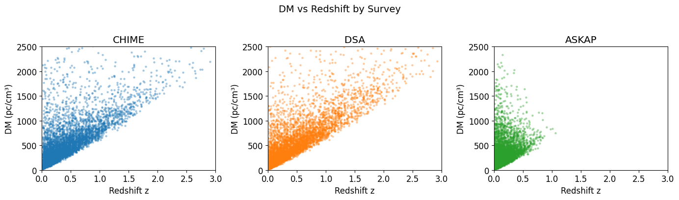
DM vs Redshift
[10]:
fig, axes = plt.subplots(1, 3, figsize=(14, 4))

for ax, (name, df), color in zip(axes, surveys.items(), colors):
    ax.scatter(df['z'], df['DMeg'], alpha=0.3, s=5, color=color)
    ax.set_xlabel('Redshift z')
    ax.set_ylabel('DM (pc/cm³)')
    ax.set_title(f'{name}')
    ax.set_xlim(0, 3)
    ax.set_ylim(0, 2500)

plt.suptitle('DM vs Redshift by Survey', fontsize=14, y=1.02)
plt.tight_layout()
plt.show()
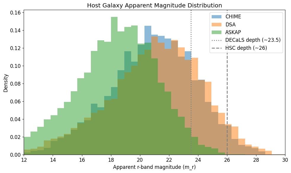
Apparent Magnitude Distributions
The apparent magnitude of the host galaxy depends on both the absolute magnitude (M_r) and the redshift.
[11]:
fig, ax = plt.subplots(figsize=(10, 6))

bins = np.linspace(12, 30, 40)
for (name, df), color in zip(surveys.items(), colors):
    ax.hist(df['m_r'], bins=bins, alpha=0.5, color=color, label=name, density=True)

# Add typical survey depth limits
ax.axvline(23.5, color='gray', linestyle=':', linewidth=2, label='DECaLS depth (~23.5)')
ax.axvline(26, color='gray', linestyle='--', linewidth=2, label='HSC depth (~26)')

ax.set_xlabel('Apparent r-band magnitude (m_r)')
ax.set_ylabel('Density')
ax.set_title('Host Galaxy Apparent Magnitude Distribution')
ax.legend()
ax.set_xlim(12, 30)
plt.tight_layout()
plt.show()
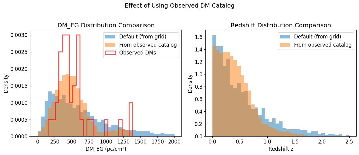
Using an Observed DM Catalog
If you have observed DM values from a specific sample, you can use them to constrain the DM distribution via kernel density estimation. This is useful when you want to simulate FRBs that match a specific observed population.
[12]:
# Example: DMs from DSA-110 observations (Connor+24)
dsa_observed_dms = np.array([
    561.50, 186.30, 335.40, 371.00, 415.90, 429.50, 586.80, 312.40,
    213.90, 597.00, 572.70, 1019.50, 576.40, 275.10, 387.80, 405.30,
    1347.10, 359.50, 319.70, 508.30, 662.30, 552.10, 789.50, 571.30,
    406.90, 1204.10, 412.00, 306.00, 547.80, 591.50, 395.10, 356.50,
    441.30, 445.20, 1371.70, 317.30, 501.50, 453.20, 723.60
])

print(f"Observed DSA DMs: N={len(dsa_observed_dms)}, median={np.median(dsa_observed_dms):.0f} pc/cm³")
Observed DSA DMs: N=39, median=445 pc/cm³
[13]:
# Generate FRBs using the observed DM distribution
df_dsa_from_catalog = generate_frbs(5000, 'DSA', dm_catalog=dsa_observed_dms, seed=42)

# Compare with default sampling
df_dsa_default = generate_frbs(5000, 'DSA', seed=42)
Loading P(DM,z) grid from /home/xavier/Projects/FRB/FRB/frb/data/DM/DSA_pzdm.npz
Sampling DM values
Sampling redshifts
Sampling host galaxy absolute magnitudes
Using Lz values to sample host galaxy absolute magnitudes
Loading P(DM,z) grid from /home/xavier/Projects/FRB/FRB/frb/data/DM/DSA_pzdm.npz
Sampling DM values
Sampling redshifts
Sampling host galaxy absolute magnitudes
Using Lz values to sample host galaxy absolute magnitudes
[14]:
fig, axes = plt.subplots(1, 2, figsize=(12, 5))

# DM comparison
ax = axes[0]
bins = np.linspace(0, 2000, 40)
ax.hist(df_dsa_default['DMeg'], bins=bins, alpha=0.5, label='Default (from grid)', density=True)
ax.hist(df_dsa_from_catalog['DMeg'], bins=bins, alpha=0.5, label='From observed catalog', density=True)
ax.hist(dsa_observed_dms, bins=bins, alpha=0.7, histtype='step', linewidth=2,
        color='red', label='Observed DMs', density=True)
ax.set_xlabel('DM_EG (pc/cm³)')
ax.set_ylabel('Density')
ax.set_title('DM_EG Distribution Comparison')
ax.legend()

# Redshift comparison
ax = axes[1]
bins = np.linspace(0, 2.5, 40)
ax.hist(df_dsa_default['z'], bins=bins, alpha=0.5, label='Default (from grid)', density=True)
ax.hist(df_dsa_from_catalog['z'], bins=bins, alpha=0.5, label='From observed catalog', density=True)
ax.set_xlabel('Redshift z')
ax.set_ylabel('Density')
ax.set_title('Redshift Distribution Comparison')
ax.legend()

plt.suptitle('Effect of Using Observed DM Catalog', fontsize=14, y=1.02)
plt.tight_layout()
plt.show()
Reproducibility
Using the seed parameter ensures reproducible results.
[15]:
# Generate two sets with the same seed
df1 = generate_frbs(100, 'CHIME', seed=12345)
df2 = generate_frbs(100, 'CHIME', seed=12345)

# Verify they are identical
print("Are the two DataFrames identical?")
print(f"  DM:  {np.allclose(df1['DMeg'], df2['DMeg'])}")
print(f"  z:   {np.allclose(df1['z'], df2['z'])}")
print(f"  M_r: {np.allclose(df1['M_r'], df2['M_r'])}")
print(f"  m_r: {np.allclose(df1['m_r'], df2['m_r'])}")
Loading P(DM,z) grid from /home/xavier/Projects/FRB/FRB/frb/data/DM/CHIME_pzdm.npz
Sampling DM values
Sampling redshifts
Sampling host galaxy absolute magnitudes
Using Lz values to sample host galaxy absolute magnitudes
Loading P(DM,z) grid from /home/xavier/Projects/FRB/FRB/frb/data/DM/CHIME_pzdm.npz
Sampling DM values
Sampling redshifts
Sampling host galaxy absolute magnitudes
Using Lz values to sample host galaxy absolute magnitudes
Are the two DataFrames identical?
  DM:  True
  z:   True
  M_r: True
  m_r: True
Using a Custom Cosmology
By default, the module uses Planck18 cosmology. You can specify a different cosmology for the distance modulus calculations.
[16]:
from astropy.cosmology import WMAP9, Planck18

# Compare apparent magnitudes with different cosmologies
df_planck = generate_frbs(1000, 'CHIME', cosmo=Planck18, seed=42)
df_wmap = generate_frbs(1000, 'CHIME', cosmo=WMAP9, seed=42)

# The DM, z, and M_r will be the same, but m_r will differ slightly
print("Comparison of apparent magnitudes with different cosmologies:")
print(f"  Planck18 median m_r: {df_planck['m_r'].median():.3f}")
print(f"  WMAP9 median m_r:    {df_wmap['m_r'].median():.3f}")
print(f"  Difference:          {(df_planck['m_r'].median() - df_wmap['m_r'].median()):.4f} mag")
Loading P(DM,z) grid from /home/xavier/Projects/FRB/FRB/frb/data/DM/CHIME_pzdm.npz
Sampling DM values
Sampling redshifts
Sampling host galaxy absolute magnitudes
Using Lz values to sample host galaxy absolute magnitudes
Loading P(DM,z) grid from /home/xavier/Projects/FRB/FRB/frb/data/DM/CHIME_pzdm.npz
Sampling DM values
Sampling redshifts
Sampling host galaxy absolute magnitudes
Using Lz values to sample host galaxy absolute magnitudes
Comparison of apparent magnitudes with different cosmologies:
  Planck18 median m_r: 21.015
  WMAP9 median m_r:    20.980
  Difference:          0.0346 mag
Calculating Detection Fractions
One common use case is to estimate what fraction of FRB hosts would be detectable given a survey magnitude limit.
[17]:
# Survey depth limits
mag_limits = {
    'Pan-STARRS': 23.2,
    'DECaLS': 23.5,
    'HSC-Wide': 26.0,
    'HSC-Deep': 27.0,
}

print("Fraction of FRB hosts detectable by survey depth:")
print("=" * 65)
print(f"{'Survey':<15} {'Limit':<8} {'CHIME':<12} {'DSA':<12} {'ASKAP':<12}")
print("-" * 65)

for survey_name, mag_limit in mag_limits.items():
    fracs = []
    for df in [df_chime, df_dsa, df_askap]:
        frac = (df['m_r'] < mag_limit).mean() * 100
        fracs.append(f"{frac:.1f}%")
    print(f"{survey_name:<15} {mag_limit:<8.1f} {fracs[0]:<12} {fracs[1]:<12} {fracs[2]:<12}")
Fraction of FRB hosts detectable by survey depth:
=================================================================
Survey          Limit    CHIME        DSA          ASKAP
-----------------------------------------------------------------
Pan-STARRS      23.2     78.0%        73.5%        96.6%
DECaLS          23.5     81.5%        76.9%        97.6%
HSC-Wide        26.0     96.7%        95.3%        99.9%
HSC-Deep        27.0     98.8%        98.1%        100.0%
Saving Generated FRBs
You can save the generated FRB population to various formats for later use.
[18]:
# Generate a sample population
df_sample = generate_frbs(10000, 'CHIME', seed=42)

# Save to different formats
# df_sample.to_csv('simulated_chime_frbs.csv', index=False)
# df_sample.to_parquet('simulated_chime_frbs.parquet', index=False)

print("Example of saving to CSV:")
print("  df_sample.to_csv('simulated_chime_frbs.csv', index=False)")
print("\nExample of saving to Parquet:")
print("  df_sample.to_parquet('simulated_chime_frbs.parquet', index=False)")
Loading P(DM,z) grid from /home/xavier/Projects/FRB/FRB/frb/data/DM/CHIME_pzdm.npz
Sampling DM values
Sampling redshifts
Sampling host galaxy absolute magnitudes
Using Lz values to sample host galaxy absolute magnitudes
Example of saving to CSV:
  df_sample.to_csv('simulated_chime_frbs.csv', index=False)

Example of saving to Parquet:
  df_sample.to_parquet('simulated_chime_frbs.parquet', index=False)
Summary
The generate_frbs() function provides a simple interface for generating realistic FRB populations:
Basic usage:
generate_frbs(n_frbs, survey)- samples from survey-specific P(z,DM) gridsCustom DM distribution: Use
dm_catalogto sample DMs from observed valuesReproducibility: Use
seedfor reproducible resultsCustom cosmology: Use
cosmoto specify a different cosmology
The generated populations can be used for:
Testing PATH analysis pipelines
Estimating host galaxy detection fractions
Studying selection effects across surveys
Planning observations
[ ]: